Neural Style Transfer with pystiche

This example showcases how a basic Neural Style Transfer (NST), i.e. image optimization, could be performed with pystiche.

Note

This is an example how to implement an NST and not a tutorial on how NST works. As such, it will not explain why a specific choice was made or how a component works. If you have never worked with NST before, we strongly suggest you to read the Gist first.

Setup

We start this example by importing everything we need and setting the device we will be working on.

import pystiche
from pystiche import demo, enc, loss, optim
from pystiche.image import show_image
from pystiche.misc import get_device, get_input_image

print(f"I'm working with pystiche=={pystiche.__version__}")

device = get_device()
print(f"I'm working with {device}")

Out:

I'm working with pystiche==1.0.1
I'm working with cuda

Multi-layer Encoder

The content_loss and the style_loss operate on the encodings of an image rather than on the image itself. These encodings are generated by a pretrained encoder. Since we will be using encodings from multiple layers we load a multi-layer encoder. In this example we use the vgg19_multi_layer_encoder that is based on the VGG19 architecture introduced by Simonyan and Zisserman [SZ14] .

multi_layer_encoder = enc.vgg19_multi_layer_encoder()
print(multi_layer_encoder)

Out:

VGGMultiLayerEncoder(
  arch=vgg19, framework=torch
  (preprocessing): TorchPreprocessing(
    (0): Normalize(mean=('0.485', '0.456', '0.406'), std=('0.229', '0.224', '0.225'))
  )
  (conv1_1): Conv2d(3, 64, kernel_size=(3, 3), stride=(1, 1), padding=(1, 1))
  (relu1_1): ReLU()
  (conv1_2): Conv2d(64, 64, kernel_size=(3, 3), stride=(1, 1), padding=(1, 1))
  (relu1_2): ReLU()
  (pool1): MaxPool2d(kernel_size=2, stride=2, padding=0, dilation=1, ceil_mode=False)
  (conv2_1): Conv2d(64, 128, kernel_size=(3, 3), stride=(1, 1), padding=(1, 1))
  (relu2_1): ReLU()
  (conv2_2): Conv2d(128, 128, kernel_size=(3, 3), stride=(1, 1), padding=(1, 1))
  (relu2_2): ReLU()
  (pool2): MaxPool2d(kernel_size=2, stride=2, padding=0, dilation=1, ceil_mode=False)
  (conv3_1): Conv2d(128, 256, kernel_size=(3, 3), stride=(1, 1), padding=(1, 1))
  (relu3_1): ReLU()
  (conv3_2): Conv2d(256, 256, kernel_size=(3, 3), stride=(1, 1), padding=(1, 1))
  (relu3_2): ReLU()
  (conv3_3): Conv2d(256, 256, kernel_size=(3, 3), stride=(1, 1), padding=(1, 1))
  (relu3_3): ReLU()
  (conv3_4): Conv2d(256, 256, kernel_size=(3, 3), stride=(1, 1), padding=(1, 1))
  (relu3_4): ReLU()
  (pool3): MaxPool2d(kernel_size=2, stride=2, padding=0, dilation=1, ceil_mode=False)
  (conv4_1): Conv2d(256, 512, kernel_size=(3, 3), stride=(1, 1), padding=(1, 1))
  (relu4_1): ReLU()
  (conv4_2): Conv2d(512, 512, kernel_size=(3, 3), stride=(1, 1), padding=(1, 1))
  (relu4_2): ReLU()
  (conv4_3): Conv2d(512, 512, kernel_size=(3, 3), stride=(1, 1), padding=(1, 1))
  (relu4_3): ReLU()
  (conv4_4): Conv2d(512, 512, kernel_size=(3, 3), stride=(1, 1), padding=(1, 1))
  (relu4_4): ReLU()
  (pool4): MaxPool2d(kernel_size=2, stride=2, padding=0, dilation=1, ceil_mode=False)
  (conv5_1): Conv2d(512, 512, kernel_size=(3, 3), stride=(1, 1), padding=(1, 1))
  (relu5_1): ReLU()
  (conv5_2): Conv2d(512, 512, kernel_size=(3, 3), stride=(1, 1), padding=(1, 1))
  (relu5_2): ReLU()
  (conv5_3): Conv2d(512, 512, kernel_size=(3, 3), stride=(1, 1), padding=(1, 1))
  (relu5_3): ReLU()
  (conv5_4): Conv2d(512, 512, kernel_size=(3, 3), stride=(1, 1), padding=(1, 1))
  (relu5_4): ReLU()
  (pool5): MaxPool2d(kernel_size=2, stride=2, padding=0, dilation=1, ceil_mode=False)
)

Perceptual Loss

The core components of every NST are the content_loss and the style_loss. Combined they make up the perceptual loss, i.e. the optimization criterion. In this example we use the feature_reconstruction_loss introduced by Mahendran and Vedaldi [MV15] as content_loss.

We first extract the content_encoder that generates encodings from the content_layer. Together with the content_weight we initialize a FeatureReconstructionOperator serving as content loss.

content_layer = "relu4_2"
content_encoder = multi_layer_encoder.extract_encoder(content_layer)
content_weight = 1e0
content_loss = loss.FeatureReconstructionLoss(
    content_encoder, score_weight=content_weight
)
print(content_loss)

Out:

FeatureReconstructionLoss(
  (encoder): VGGMultiLayerEncoder(layer=relu4_2, arch=vgg19, framework=torch)
)

We use the gram_loss introduced by Gatys, Ecker, and Bethge [GEB16] as style_loss. Unlike before we use multiple style_layers. The individual GramOperator s can be conveniently bundled in a MultiLayerEncodingOperator.

style_layers = ("relu1_1", "relu2_1", "relu3_1", "relu4_1", "relu5_1")
style_weight = 1e3


def get_style_op(encoder, layer_weight):
    return loss.GramLoss(encoder, score_weight=layer_weight)


style_loss = loss.MultiLayerEncodingLoss(
    multi_layer_encoder, style_layers, get_style_op, score_weight=style_weight,
)
print(style_loss)

Out:

MultiLayerEncodingLoss(
  encoder=VGGMultiLayerEncoder(arch=vgg19, framework=torch), score_weight=1000
  (relu1_1): GramLoss(score_weight=0.2)
  (relu2_1): GramLoss(score_weight=0.2)
  (relu3_1): GramLoss(score_weight=0.2)
  (relu4_1): GramLoss(score_weight=0.2)
  (relu5_1): GramLoss(score_weight=0.2)
)

We combine the content_loss and style_loss into a joined PerceptualLoss, which will serve as optimization criterion.

perceptual_loss = loss.PerceptualLoss(content_loss, style_loss).to(device)
print(perceptual_loss)

Out:

PerceptualLoss(
  (content_loss): FeatureReconstructionLoss(
    (encoder): VGGMultiLayerEncoder(layer=relu4_2, arch=vgg19, framework=torch)
  )
  (style_loss): MultiLayerEncodingLoss(
    encoder=VGGMultiLayerEncoder(arch=vgg19, framework=torch), score_weight=1000
    (relu1_1): GramLoss(score_weight=0.2)
    (relu2_1): GramLoss(score_weight=0.2)
    (relu3_1): GramLoss(score_weight=0.2)
    (relu4_1): GramLoss(score_weight=0.2)
    (relu5_1): GramLoss(score_weight=0.2)
  )
)

Images

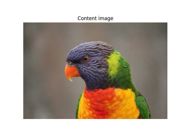
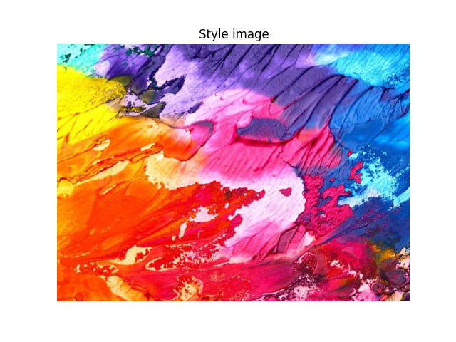
We now load and show the images that will be used in the NST. The images will be resized to size=500 pixels.

images = demo.images()
images.download()
size = 500

Note

ìmages.download() downloads all demo images upfront. If you only want to download the images for this example remove this line. They will be downloaded at runtime instead.

Note

If you want to work with other images you can load them with read_image():

from pystiche.image import read_image

my_image = read_image("my_image.jpg", size=size, device=device)

content_image = images["bird1"].read(size=size, device=device)
show_image(content_image, title="Content image")

style_image = images["paint"].read(size=size, device=device)
show_image(style_image, title="Style image")

Neural Style Transfer

After loading the images they need to be set as targets for the optimization criterion.

perceptual_loss.set_content_image(content_image)
perceptual_loss.set_style_image(style_image)

As a last preliminary step we create the input image. We start from the content_image since this way the NST converges quickly.

Note

If you want to start from a white noise image instead use starting_point = "random" instead:

starting_point = "random"
input_image = get_input_image(starting_point, content_image=content_image)

starting_point = "content"
input_image = get_input_image(starting_point, content_image=content_image)
show_image(input_image, title="Input image")

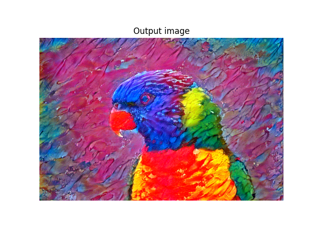
Finally we run the NST with the image_optimization() for num_steps=500 steps.

In every step the perceptual_loss is calculated nd propagated backward to the pixels of the input_image. If get_optimizer is not specified, as is the case here, the default_image_optimizer(), i.e. LBFGS is used.

output_image = optim.image_optimization(input_image, perceptual_loss, num_steps=500)

Out:

Image optimization: 100%|██████████| 500/500 [01:27<00:00,  5.69it/s, loss=1.078e+01]

After the NST is complete we show the result.

show_image(output_image, title="Output image")

Conclusion

If you started with the basic NST example without pystiche this example hopefully convinced you that pystiche is a helpful tool. But this was just the beginning: to unleash its full potential head over to the more advanced examples.

Estimated memory usage: 2300 MB